Test results allow the TA to identify failures, but they also provide feedback to the TA to help improve defect detection effectiveness. Some commonly used techniques to analyze test results are described below.

Predicted versus actual defect cluster analysis . A few components usually contain most defects (see ISTQB-CTFL, v4.0.1, Section 1.3). After testing, the TA can identify the actual defect-prone areas and compare predicted versus actual defect clusters. In the case of discrepancies, more rigorous testing may be applied to areas where more defects were found than expected. When determining the clusters, measurable criteria should ensure clarity and consistency (e.g., defect density and defect severity). Among these criteria, the severity of the defects should play a significant role. Small clusters of critical or major defects are usually more important (i.e., need more rigorous testing) than larger clusters of minor or cosmetic defects.

Defect detection percentage (DDP) analysis . DDP is one of the most important test effectiveness measures for a test level. When calculating DDP, the number of escaped defects should be limited to those that the test level under consideration could have detected. Clear boundaries for defect counting, such as temporal limits (e.g., defects found within a defined time frame after release) and exclusion criteria (e.g., defects in third-party components or specific customer environments), should be established to ensure consistency. A low DDP for a given test level indicates a high percentage of escaped defects, meaning defect detection is ineffective. In such a case, the TA should analyze the reasons and propose measures to improve it, making the test level more focused and rigorous. The DDP is best divided by severity levels, as the priority of reducing escaped defects usually depends on their severity.

Structural coverage analysis assesses the extent to which tests have exercised specific areas of the test object. Identifying low-coverage areas allows the TA to target test efforts in those areas. Increasing their coverage helps to discover new, previously escaped defects. Structural coverage such as statement coverage, branch coverage, or neuron coverage is usually measured with test tools. When selecting the additional areas to be covered, their risk levels should be considered.

Test gap analysis assesses the extent to which tests have exercised recent code changes. This allows the TA to focus additional test effort in areas that are especially error prone (i.e., new changes that have not been tested at all) instead of targeting all areas that have low coverage (e.g., code that has not changed in a long time and has been tested for previous releases).

Defect arrival pattern analysis . The number or density of defects found in successive phases of a project (e.g., iterations) can be compared with patterns that describe the theoretical distribution of these values over time. A classic example of a defect arrival pattern is the Rayleigh model (Elsayed, 2021). It has a single peak and is skewed to the right, showing that the expected number of defects found first increases in time and, after reaching its maximum value, drops down slowly towards zero. Based on the analysis of such a pattern, it is possible to infer the strength of existing test cases and the potential for their improvement. For example, suppose defect detection remains at a constant, low level when the pattern suggests it should be increasing. In that case, it may mean that the existing tests are too weak and unable to detect additional defects.

The analytical methods described above use various defect-related metrics, such as the number of defects or DDP. These metrics are calculated based on the test results (e.g., number of tests passed/failed), defect reports, and structural metrics (e.g., code coverage or defect density). Note, however, that these metrics are not always as easy to read from the test results as they may seem. For example, the number of failed tests is not necessarily the same as the number of defects detected by these tests. To calculate the actual number of defects detected, the results of the debugging process must be carefully analyzed because the relation between test results and defects can be many-to-many. Several tests may detect the same defect or one test may detect several defects. Moreover, the severity of the defects may differ from the criticality of the tests, as a critical test case may fail due to a cosmetic defect.

Objective metrics from tools are designed and collected based on the needs of the test team and other stakeholders. Test tools mostly capture valuable real-time data and reduce data collection efforts. This data is used to manage the overall test effort and identify areas for optimization.

Different tools are focused on collecting different types of data. Examples of these include:

• Test management tools can supply a variety of different metrics related to available test items, tests, planned tests as well as current and passed test execution status (e.g., passed, failed, skipped, blocked or planned)
• Requirements management tools deliver traceability regarding requirements coverage by passed and failed test cases
• Defect management tools can provide defect information such as status, severity, priority and defect density of test items. Other valuable data, such as the defect detection percentage, the test levels at which defects are introduced and detected defect lead time help to drive process improvement, but may not all be provided solely by the defect management tool.

• Static analysis tools, among others, supply metrics related to code complexity
• Performance testing tools can supply valuable information such as response times and failure rates under peak loads
• Code coverage tools help to understand which parts of the test object have been exercised by testing
• Although test tools can be used to collect metrics, they should also monitor themselves. In this context the quality of the test process can be measured (e.g., the number of defects found with and without tools and requirements coverage)
• Test efficiency (e.g., duration of test execution and number of executed tests)

More details on the collection and usage of metrics can be found in Section 2.1 of this syllabus, Test Metrics.

The information on a defect report should suffice for the following purposes:

• Management of the defect report through the defect lifecycle
• Assessment of overall project status, especially in terms of product quality, and test progress
• Assessment of the status of a product increment in terms of product quality
• Assessment of process capability

The information needed for defect management and project status can vary depending on when the defect is detected in the SDLC. In addition, defect reports related to non-functional quality characteristics may need more information (e.g., load conditions for performance issues). However, the core information gathered should be consistent across the SDLC and ideally across all projects in an organization to allow for meaningful comparison of defect data throughout the project and across all projects.

Many data items can be collected in a defect report. The test manager should decide which information is appropriate for effective defect management for a given project context. Due to the fact that each additional attribute increases the time spent on defect reporting and may increase confusion by the person who is entering the defect report, it is advisable to only collect data that is needed for defect management in the given context and/or will be used for process improvement.

To manage the defect report in most environments, the following are mandatory:

• A defect title with a short summary of the anomaly
• A detailed description of the anomaly preferably including steps to reproduce the failure
• Severity of the impact on the system under test and/or the product stakeholders
• Priority to fix the anomaly

Additional important data items are often created by the defect management tool:

• Unique identifier for the defect report
• Date/time of creation of the defect report

• Name of the person who discovered and/or reported the anomaly
• Project and SDLC phase in which the anomaly was discovered
• Current state of the defect report
• Current owner (i.e., the person currently assigned to work on the defect)
• Change history such as the sequence of actions, including date/time information, taken by project team members to isolate, repair and confirm the defect as fixed
• References (e.g. to test case, to connected defects).

Depending on context, further information (e.g. traceability) may also be collected in a defect report (see the ISO/IEC/IEEE 29119-3 for more information). The following bullet points group the information according to the intended purpose:

• To help defect resolution : The subsystem or component in which the defect lies, the specific test item and its release number in which the anomaly was observed or the test environment in which the defect was observed
• To assess the overall project status: Information to monitor progress, (e.g., risks, costs, opportunities, and benefits associated with fixing or not fixing the defect, a description of any available workaround, or requirements affected by the defects)
• To assess the status of a product increment in terms of product quality: The type of defect (usually corresponding to a defect taxonomy), the work product in which the defect was introduced, or the quality characteristic/sub-characteristic affected by the defect
• To assess the process capability : Information to monitor the effectiveness and efficiency of the development processes (e.g., the SDLC phase of introduction, detection, and removal for the defect or defect root cause)

As discussed in Section 2.3.5 of this syllabus, Defect Report Information, defect reports can be useful for project status monitoring and reporting. While the implications of metrics on the test process are primarily addressed in the Expert Test Management Syllabus, at the Advanced Test Management Level, test managers should be aware of what defect reports mean to assessing the capability of the software development and testing processes.

In addition to the test progress monitoring information mentioned in this syllabus, in section 2.1.2, Monitoring, Control and Completion, and in section 2.1.3, Test Reporting, defect information should support process improvement initiatives as discussed during retrospectives. Examples include:

• Using information about the phases of introduction, detection, and removal of defects to assess phase containment and/or perform cost of quality analysis with the aim of suggesting ways to improve defect detection effectiveness in each phase and minimize the cost associated with defects
• Using information about the phase of introduction for analysis of the phases in which the largest number of defects are introduced, to enable targeted improvements for defect prevention
• Using defect root cause information to determine the underlying reasons for defect introduction, to enable process improvements that reduce the total number of defects
• Using defect location information to perform defect cluster analysis, to better understand technical risks (for risk-based testing) and to enable re-factoring of troublesome components
• Using information about re-opened defects to assess the quality of debugging implementations
• Using information about duplicate and rejected defects to assess the quality of the defect report creation
• Enable process improvements that reduce the total number of defects by introducing pro-active measures to avoid errors upfront

The use of metrics to assess the test process effectiveness and efficiency is discussed in the Expert Test Management Syllabus.

In some cases, teams decide not to track defects found during some or all phases of the SDLC. While this is often carried out in the name of efficiency and for the sake of reducing process overhead, it greatly reduces visibility into the process capabilities of software development and testing. This makes the improvements suggested above difficult to carry out due to a lack of reliable support data.

If an analytical approach to improvement is being used (Chapter 4), the current situation may be analyzed by applying concepts such as:

• Systems Thinking [Weinberg 92]
• Tipping Points [Gladwell]

Systems Thinking helps analyze the relationships between different system (process) components and to represent those relationships as stable (“balancing”) loops or reinforcing loops. A reinforcing loop may have a negative effect (“vicious circle”) or a positive effect (“virtuous circle”).

Tipping Points help identify specific points in a system where a small, well-focused improvement may break a vicious circle and set off a chain reaction of further improvements.

When a model-based approach (Chapter 3) for test process improvement is followed, a comparison is made between the process maturity of the current situation and the desired objectives defined at the initializing phase.

Where appropriate benchmarks are available, these should be used in evaluating results. The following benchmarks may be used, where available:

• Company-based, representing an entire organization
• Industry-based, where possible relating to the same business segment
• Project-based, where the comparison is made with a specific project that is regarded as meeting the desired objectives

Where key performance indicators have been established (see Section 4.4 and Section 6.2.2), these should be incorporated into the analysis. For example, if the Defect Density Percentage (DDP) has fallen below the required level, an analysis of faults found in production should be performed to evaluate their sources.

The result of the evaluation should provide sufficient information with which to define recommendations and support the planning process (see Sections 6.3.7 and 6.4 below).

Each phase of the SDLC should include activities to detect and remove potential defects. For example, static testing techniques (i.e. reviews and static analysis) can be used on design specifications, requirements specifications and code prior to delivering those work products into subsequent activities. The earlier each defect is detected and removed, the lower the overall cost of quality for the product. Cost of quality is minimized when each defect is removed within the same phase in which it was introduced (i.e., when the software process achieves perfect phase containment).

During static testing we search for defects. During dynamic testing the presence of a defect is revealed when it causes a failure, which results in a discrepancy between the actual results and the expected results of a test (i.e., an anomaly). In some cases, a false-negative result occurs when the tester does not observe the anomaly. When an anomaly is observed, further investigation should be performed. This investigation usually starts with completing a defect report in accordance with the defined test and defect management process. A failed test does not always result in the creation of a defect report. (For example, in test-driven development, where component tests, usually automated, are used as a form of executable design specification). Until the development of the component is complete, some or all of the tests must initially fail. Until the development of the component is complete, some or all of the tests must initially fail. Therefore, the result of such a test is not necessarily caused by a defect and is typically not tracked via a defect report.

A defect report progresses along a workflow (for simplicity and consistency with most defect management tools we will further use the term “defect workflow”) and moves through a sequence of defect states. In most of these states, one person owns the defect report and is responsible for carrying out a task (e.g., analysis, defect removal, or confirmation test). The following diagram represents a simple defect workflow:

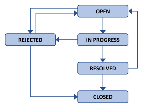
Figure 2: A Simple Defect Workflow

A simple defect workflow may cover the following defect states:

• OPEN (may be called NEW): The initial state when the defect report is created.
• IN PROGRESS: The team is working on the defect report analysis and/or fix.
• REJECTED: A defect report is rejected by the person who processed it (usually a developer or an analyst). There may be many reasons for rejection (e.g., invalid information, incorrect test, duplicate defect report) and this information is added to the defect report.
• RESOLVED (may be called FIXED, READY FOR RETEST): A tester runs a confirmation test often following the steps to reproduce the failure from the defect report itself to determine whether the fix has indeed resolved the defect.
• CLOSED: The defect report has reached its terminal state, and no further work is intended to be done. The tester transitions the defect report to this state either after a successful confirmation test or to acknowledge rejection of the defect report.

A simple defect workflow is used in many organizations and is extended by the use of other defect states relevant for a given context (e.g., RE-OPENED, ACCEPTED, CLARIFICATION, or DEFERRED).

The defect workflow may vary in different organizations in terms of different names of the defect states, rules for transitions among defect states and roles responsible for tasks in given defect states. Often the defect workflow is more simple in Agile software development than in sequential development models. The defect workflow should be adapted to a given context. When designing the defect workflow, it is advisable to respect several good practices:

• If possible, the defect workflow should be defined organization-wide to provide unified defect management across all projects
• Duplicate and false-positive defects should be represented by a separate state or a combination of the REJECTED status with choosing the reason for rejection. They may be helpful in further defect analyses with the aim of improving the test process.

• It is recommended to use only one terminal state (e.g., CLOSED). The transition to this state often requires choosing a reason for closure, useful for process assessment and process improvement activities.
• The names of states in the defect workflow should be the same as for analogous states used for other entities (e.g., user stories and test tasks) to simplify working with them.
• Consecutive defect states should belong to different responsible roles. If two or more consecutive states belong to the same responsible role, there should be a good reason (e.g., to measure the time spent in a defect state).
• Each defect state, except for the terminal state, should have more than one outgoing transition to allow the responsible role a decision regarding the next step. Exceptions of this rule should be justified (e.g., to monitor time spent on a given activity).
• The set of attributes required to be entered when performing a state transition should be limited to those which give substantial value to defect management.